Multifamily Affordability Gap Index and Post-2025 HUD-AMI Impacts

Introduction

Housing affordability remains a pressing concern in the United States, even as we enter the post-2025 landscape with updated income data from the U.S. Department of Housing and Urban Development (HUD). Recent reports highlight a widening gap between what households earn and what they must pay for housing, particularly in the rental market. Nationwide, renters in 2025 need to earn over $80,000 to comfortably afford the typical apartment, about $20,000 more than just five years prior. The National Low Income Housing Coalition notes a shortage of 7.1 million affordable rental homes for the lowest-income Americans– a stark indicator of the housing affordability gap. This article introduces the concept of a Multifamily Affordability Gap Index, explaining how it is constructed and why it’s an especially useful tool after the 2025 HUD Area Median Income (AMI) updates. We will explore how this index behaves in key U.S. markets (Austin, Miami, Phoenix, Raleigh-Durham, Denver, Atlanta, etc.), and analyze its role in real estate investment decisions and public policy. In addition, we compare the index to traditional measures (cost-burden ratios, rent-to-income ratios, LIHTC income limits) and discuss how factors like design, zoning, and construction costs influence housing affordability. A detailed case study with a modeled example is included to illustrate these concepts in practice.

Why focus on 2025? Because the landscape of affordable housing development strategies is shifting in response to new data and post-pandemic trends. HUD’s 2025 AMI update has reset income benchmarks across the country, influencing everything from LIHTC (Low-Income Housing Tax Credit) eligibility to rent limits on existing affordable units. Meanwhile, market rents in many cities surged during the early 2020s. The result is a dynamic where in some high-growth metros, even middle-income families are feeling the housing affordability gap 2025 has brought. For investors and developers, understanding this gap is crucial for identifying multifamily investment opportunities USA that are both financially viable and socially impactful. And for policymakers, a clear measure of the gap informs better targeting of resources and zoning reforms. In the sections below, we define the Multifamily Affordability Gap Index and delve into its construction, use cases, and insights for various stakeholders in this new context.

Defining the Multifamily Affordability Gap Index

The Multifamily Affordability Gap Index is a conceptual metric that quantifies the difference between housing costs in the multifamily rental market and what local households can afford to pay. In simple terms, it measures how far apart the market-rate rent for an apartment is from the affordable rent given local income levels (often benchmarked by HUD’s AMI). This index is particularly relevant for the “missing middle” – households who earn too much to qualify for traditional low-income housing subsidies but still struggle to afford market-rate rents. As RSM US describes, the widening divide between subsidized low-income housing and market-rate rentals is commonly referred to as the “affordability gap,” especially affecting essential workforce households earning roughly 60% to 120% of AMI. The Affordability Gap Index aims to put a number on that divide.

At its core, the index can be thought of as a rent-to-income ratio or difference, standardized for a given area. For example, an index value of 1.0 (or 100 when expressed as a percentage) might indicate that the median-income household in an area would have to spend exactly 30% of its income to afford the median rent (meeting the standard definition of affordability). A value above 1.0 (>100%) would mean the median rent is above the affordability threshold for the median income, indicating a gap. A value below 1.0 (<100%) means the median rent is below the 30%-of-income affordability threshold for that area’s median income (indicating relatively better affordability at the median). In essence, the index synthesizes what portion of local income a typical rental consumes, or conversely, how much income is “missing” for housing to be affordable.

Why introduce a new index when cost-burden metrics exist? Traditional measures like the cost-burden ratio (the percentage of income a household spends on housing) are indeed part of this calculation – for instance, we often cite that spending above 30% of income on rent indicates an affordability problem. However, those measures usually describe household-level situations or the share of households above a threshold, rather than providing a single comprehensive indicator for a market. The Affordability Gap Index, by contrast, aggregates information into one figure that can be tracked over time or compared across markets. It is a type of affordable housing index focused specifically on multifamily rentals and is designed to be intuitive: if the index rises, housing is becoming less affordable relative to incomes (the gap is widening); if it falls, housing is becoming more affordable or incomes are catching up.

Crucially, post-2025 HUD AMI updates make this index especially useful now. HUD’s AMI is recalculated annually and is a linchpin for affordable housing programs. In 2025, many areas saw significant increases in their AMI figures – on average about 6.2% higher than the previous year, with 27% of areas hitting HUD’s cap of a 9.2% increase. This means in many regions, the baseline of what’s considered “median income” jumped notably. A higher AMI typically raises the income thresholds for housing programs and can theoretically make rents more affordable (since households have more income on paper). But if market rents have risen even faster, the affordability gap may actually have grown. In fact, from 2020 to 2025, typical U.S. rents rose about 28.7% while median household income rose only ~22.5%. The gap index helps capture the net effect of these changes: it reflects post-HUD update conditions by incorporating the latest income data against current rent levels.

To illustrate, consider a region where the 2025 AMI update raised the median income substantially. If landlords also increased rents significantly, the index might show little improvement or even a worse affordability ratio. Conversely, in an area where incomes rose and rent growth cooled, the index would register an improvement (smaller gap). By continuously tracking this index, stakeholders can gauge whether real estate investment post-HUD update is becoming more or less risky from an affordability standpoint.

How the Index Is Constructed: Metrics and Data Sources

Constructing a Multifamily Affordability Gap Index involves a few clear steps and reliable data inputs. It is meant to be repeatable with clear metrics, so that investors, developers, or policymakers can calculate and monitor it for their market of interest. Below is a breakdown of how such an index can be built:

1. Gather Local Income Data (HUD AMI): Start with the Area Median Income (AMI) for the geography in question, as determined by HUD for the current year. HUD publishes Median Family Income estimates for each metropolitan area (often based on a family of four) and then provides income limits at various percentages of AMI. For example, in 2025, the Austin-Round Rock, TX MSA had a HUD median family income of $133,800 (for a family of four). This figure (100% AMI) serves as the benchmark for local earning capacity. Similar data for Miami’s metro (Miami-Miami Beach-Kendall HMFA) shows a 2025 median family income around $123,900 (implied by a very-low-income limit of $61,950, which is 50% AMI). HUD’s AMI figures are widely used and updated annually (effective April each year), reflecting the latest available economic data.

2. Determine “Affordable Rent” from Income: Using the chosen income level, calculate the maximum affordable housing cost. The standard criterion is that housing is affordable if it costs no more than 30% of gross income. So, if we use the median income (100% AMI) for the index, the monthly affordable rent = 0.3 × (AMI ÷ 12). For instance, a $120,000 annual income translates to $10,000 per month, and 30% of that is $3,000 per month as an affordable rent threshold. In Austin’s case (AMI $133,800), 30% of monthly income is about $3,345 – meaning a family at the median income could “afford” roughly that in rent without being cost-burdened. If analyzing a different segment (say 80% of AMI, often considered moderate or workforce income), the same calculation is applied to that income level. The index can be constructed for different income benchmarks depending on what question we want to answer (e.g., gap for median-income households, or gap for moderate-income households). Often, 100% AMI is used to gauge overall market affordability, while 60% or 80% AMI might be used to gauge workforce housing affordability.

3. Obtain Local Market Rent Data: Next, we need the typical cost of multifamily housing in that market. This can be represented by median rent or an index like the Zillow Observed Rent Index (ZORI) for a given metro, which blends various unit types into a single median-like figure. Alternative sources include HUD’s Fair Market Rents (FMRs) for standard unit sizes, or industry reports from sources like Realtor.com or Apartment List. The key is to have a clear, current figure for what a “typical” rental unit commands in the market. For example, Zillow’s data showed that in April 2025 the median listed rent nationally was about $2,024 per month. City-specific figures were: Austin around $1,721, Miami around $2,749, Phoenix about $1,853, Raleigh roughly $1,761, Denver about $1,972, and Atlanta about $1,919 per month, to name a few. These rent figures represent the market-rate cost side of the equation.

4. Calculate the Affordability Gap: With an affordable rent threshold (from step 2) and the actual market rent (from step 3), the gap can be quantified. There are a couple of ways to express it:

   • Dollar Gap: Simply subtract the affordable rent from the market rent. A positive value means market rent exceeds what is affordable at the chosen income level – this dollar amount is the monthly affordability gap per unit. For example, if a household can afford $2,000 in rent but the going rent is $2,500, the gap is $500 per month. If this number is negative, it means the target income level can afford more than the current rent (no gap for that income level).

   • Index or Ratio: Divide the market rent by the affordable rent to get a ratio. In the example above, $2,500 / $2,000 = 1.25, or 125%. We might call this Affordability Gap Index = 125 (meaning market rent is 125% of the affordable level for that income). An index of 125 signifies a substantial gap; an index of 100 would signify parity; an index of 80 (market rent is 80% of affordable threshold) would indicate strong overall affordability for that income level. This ratio can also be inverted to express required income as a percentage of actual income, but for simplicity we’ll stick to rent-based expression here.

5. Incorporate Additional Factors (if needed): The simplest form of the index uses income vs. rent as above. However, some formulations of an affordability gap consider cost of housing production as well, especially from a developer’s perspective. For instance, the Colorado Housing Finance Authority (CHFA) defines the affordability gap in development terms as “the difference between the cost to produce and operate a rental property, and the financing that can be supported by rental income from that property.”. This essentially asks: if it costs $X to build and run an apartment unit, but the rent that local tenants can pay only supports a financing of $Y, the difference $X–$Y is the funding gap requiring subsidy or concession. In constructing an index, one could integrate construction cost metrics (e.g. cost per unit, required rent per unit given construction cost) to reflect long-term feasibility. For example, if in a given city an average new multifamily unit costs $250,000–$300,000 to develop (typical for an apartment in a mid-rise building), a developer might need to charge roughly $2,100–$2,500 in monthly rent (assuming standard financing) to break even. If local median incomes only support, say, $1,800 in rent, that $300–$700 shortfall per month per unit is the development affordability gap. While this adds complexity, it’s a useful extension when the goal is to inform policy on how much subsidy or cost reduction is needed to make new housing attainable.

   
   

In practice, most users of the Affordability Gap Index will focus on the income vs. market rent approach, because data for that is readily available and it directly speaks to households’ experience. Table 1 below provides a modeled example of how to calculate the gap for a moderate-income household in two different cities, using 2025 data:

Table 1: Affordability Gap Example for a Moderate-Income (80% AMI) Family in 2025

City	2025 Income @ 80% AMI (4-person)	Affordable Rent (30% of income)	Typical Market Rent (Monthly)	Monthly Gap (Market – Affordable)	Gap as % of Affordable Rent
Austin, TX	$104,200vper year	$2,605 per month	~$1,721 per month	–$884 (surplus income)	–34% (Market is 66% of affordable)
Miami, FL	$99,100 per year	$2,478 per month	~$2,749 per month	+$271 (shortfall)	+11% (Market is 111% of affordable)

Sources: HUD FY2025 income limits (80% of Area Median Income); Zillow Observed Rent Index for April 2025

In the Austin example, a household earning 80% of the median income could afford roughly $2,600 in rent, which is well above the typical asking rent of ~$1,721. This implies no affordability gap at that income level – in fact, such a household would be spending only about 20% of its income on the median apartment, well under the 30% threshold. By contrast, in Miami, a household at 80% AMI (around $99K annual income for a family of four) could afford about $2,478 in rent, but the median rent is about $2,749, resulting in a gap of roughly $271 extra per month needed. The Affordability Gap Index for these scenarios could be expressed as ~0.66 for Austin and ~1.11 for Miami (if we use affordable rent as baseline 1.0). In other words, Austin’s moderate-income families face essentially no affordability gap for a typical unit, while Miami’s face an 11% gap even at a relatively decent income level. This example underscores how dramatically the index can vary between markets, and why a one-size-fits-all national view of “affordable housing” often misses local nuances.

Why the 2025 HUD AMI Updates Matter for Affordability Metrics

Before diving into specific markets, it’s important to highlight why we keep mentioning the post-2025 HUD AMI updates and their impact. Each year, HUD recalibrates the Area Median Income based on the latest available data (largely from the American Community Survey, with some adjustments). For 2025, this update was notable in a few ways:

• Significant Income Changes: Many metro areas saw substantial increases in their AMI. The average increase was 6.2%, but a considerable share of areas (about 27%) hit a cap of +9.2%. HUD imposed a 9.2% cap to prevent extremely large jumps, given that the national median income was estimated to have risen 4.6% and HUD allows up to double that percentage under certain rules. For high-growth metros, this cap means the official income stats understate what may be happening on the ground. (If local incomes jumped 12%, HUD’s limits would still only rise 9.2%.) For our Affordability Gap Index, using the HUD-capped AMI might make the gap look a bit larger than if we had actual uncapped incomes — but since HUD AMI is the basis for program eligibility and widely used, it makes sense to use it in calculations, keeping in mind the cap effect.

• Alignment with Post-Pandemic Reality: The 2025 update is one of the first to fully incorporate the unusual economic shifts of the early 2020s (pandemic job losses, rapid wage growth in some sectors, inflation in others). In some regions, median income actually dropped or stalled in earlier years, then rebounded. HUD’s methodology smoothed some of these swings, but 2025’s numbers are closer to a new equilibrium. This means when we compare housing affordability gap 2025 to prior years, we’re seeing a clearer picture of where things have settled after the volatility. Some previously affordable-feeling markets suddenly look less so because incomes didn’t keep pace with housing costs.

• Impacts on Programs and Households: HUD AMI updates directly affect LIHTC income limits, Section 8 vouchers, HOME program rents, and other affordable housing programs. For example, if AMI rises, the income ceiling for a 60% AMI restricted unit rises, allowing slightly higher rents on those units (since LIHTC maximum rents are tied to AMI). In 2025, 71% of areas saw income limit increases above 5% and over 40% of areas saw increases above 8%. This translates into higher income eligibility for families (helping some qualify who previously earned slightly too much) and potentially higher rents collectable on affordable units (improving project revenues). For middle-income households not in any program, a higher AMI doesn’t put money in their pocket, but it might influence local policy (e.g. inclusionary zoning thresholds or what is considered “workforce housing”). The Affordability Gap Index, by updating its income input, captures these shifts. If AMI jumped but rents remained flat, the gap index would improve, signaling better affordability. If both AMI and rents jumped or rents outran AMI, the index would worsen.

In summary, 2025 marks a pivotal recalibration point. The Affordability Gap Index, when computed with the latest AMI, gives an up-to-date measure of the challenge. It also sets a baseline for the coming years – we can watch how this index changes as new housing supply comes online, as interest rates or inflation affect incomes, and as policies react to the current conditions. For investors and developers, knowing the post-2025 HUD AMI context is crucial: it tells you how much official income growth has occurred in your market (which might justify rent increases in pro formas or conversely signal a cap has been hit). For instance, in many Texas markets, incomes hit the 9.2% cap, indicating very strong growth – but if your project counted on even more income growth for affordability, that extra isn’t reflected in HUD stats (though actual residents might be earning more). On the other hand, if a market’s AMI barely increased, it could be a warning sign that rent growth might outstrip incomes (a red flag for affordability and for rent growth potential). Thus, integrating the HUD update into an index provides a grounded, data-driven foundation for assessing multifamily investment opportunities in the USA as of 2025 and beyond.

Market Spotlight: Affordability Gap Index in Key 2025 U.S. Markets

Let’s examine how the Multifamily Affordability Gap Index plays out in several financially and strategically attractive U.S. markets in 2025+. These include high-growth metros often seen as magnets for both population inflows and investor interest: Austin, Miami, Phoenix, Raleigh-Durham, Denver, and Atlanta. Each of these cities has a strong economy and robust demand for multifamily housing, but each also faces unique affordability challenges. We’ll discuss the index in each city, using data on typical rents and incomes, and explain what it means for that market’s housing conditions.

• Austin, TX: Austin is a tech-boom town that experienced rapid population and income growth in the past decade. As a result, its affordability gap index is relatively favorable at the median income level. According to Zillow’s analysis, the typical rent in Austin around April 2025 was about $1,721 per month. Meanwhile, the median household income in the Austin metro is quite high – Austin’s HUD AMI for a family of four in 2025 is $133, and even the average household income among renters (often lower than owners) is well above the U.S. norm at around $91. These high incomes mean that Austin renters spend only ~20% of their income on a typical apartment on, well under the 30% affordability threshold. In index terms, if we use median income, Austin’s index comes out to roughly 0.66 (or 66%) – signaling a surplus of income relative to median rent costs. Practically, this means a median-income household in Austin has room to spare in their housing budget; they could afford a more expensive place if needed. However, this doesn’t mean Austin has no affordability issues. The city’s cost of living, including housing, has soared, and those gains have been partially masked by the influx of higher-income residents (tech workers, etc.). Not everyone is a beneficiary of the high wages. In fact, Zillow noted that in Austin a renter needs to earn about $68,840 annually to afford the typical rent comfortably. The encouraging news is that Austin’s median incomes are above that (hence the 20% rent-to-income figure), but lower-income segments are still strained. Austin’s needed income for median rent rose about 17.6% from 2020 to 2025, indicating that rent growth outpaced many people’s pay increases. For investors, Austin’s smaller affordability gap at the median suggests a robust market where many renters can pay the rent – a positive for Class A developments and rent growth potential. For policymakers, the focus may be on targeted affordability for those not in the high-earning cohort, as the general metrics make the city look more affordable than the reality for, say, service workers. Austin has been experimenting with affordable housing development strategies like loosening zoning (allowing ADUs and higher density in some areas) and leveraging public-private partnerships to create mixed-income projects, aiming to keep the gap from widening further.

• Miami, FL: Miami is in many ways the inverse scenario to Austin. It’s a high-demand market (fueled by migration, international investment, and limited land for expansion) but with comparatively lower local median incomes, creating one of the largest affordability gaps in the country. By early 2025, Miami’s typical rent was about $2,749 per month – among the highest outside of New York and California. Yet, the median household income in the Miami metro area is much lower; many workers are in tourism, hospitality, and service sectors which haven’t seen tech-level wage gains. Zillow’s data showed that Miami renters would need to earn around $109,962 per year to afford the median rent without exceeding 30% of income. However, the actual median income in Miami is nowhere near that; a typical household would be spending about 40.4% of its income on the median rental. This translates to an Affordability Gap Index of roughly 1.35 (135%) for Miami at median values – meaning the median rent is 135% of what the median income can comfortably support. Put differently, the median Miami household falls short of affording a median-priced apartment by a wide margin. It’s no surprise that Miami tops the list of cost-burdened cities; it has one of the highest rent-to-income ratios in the nation. This gap has been rapidly widening – Zillow found the required income to afford rent in Miami jumped 54% since 2020, thanks to rent hikes far outpacing income growth. The consequence is evident: many Miami residents are doubling up, commuting from cheaper areas, or simply paying far more than 30% on housing (if they can manage it at all). For investors, Miami’s huge gap can be a double-edged sword. On one hand, high rents signal strong demand and willingness to pay (often bolstered by wealth migration into South Florida). On the other hand, the local renter pool’s ability to pay is maxed out – meaning future rent growth may be constrained unless incomes rise or new higher-income renters move in. It also signals potential for multifamily investment opportunities in the workforce housing segment: there is acute need for units that are affordable to middle-income earners. Public entities in South Florida are indeed responding; for example, Miami-Dade County has initiatives to incentivize mixed-income developments and the Miami city government is exploring zoning changes to allow greater density and inclusionary zoning in some neighborhoods. The Affordability Gap Index highlights why: with even 80%-100% AMI families facing rent gaps (as seen in Table 1, where an 80% AMI family in Miami is short by about $270 a month for a median unit), the policy focus is expanding to include moderate-income housing, not just the very poor. Miami’s case study underscores the role of the index in public policy design – it’s a clear call to action that traditional affordable housing (targeted at 50-60% AMI) isn’t enough; strategies must also address those moderate-income households slipping into the gap.

• Phoenix, AZ: Phoenix has been a fast-growing market, popular with both retirees and young families, and it saw an explosive growth in housing demand (and prices) during the early 2020s. By 2025, Phoenix’s housing affordability is middling – better than coastal cities, but worse than historically. The Zillow data put Phoenix’s typical rent at about $1,853 per month, with an income of $74,100 needed to afford that comfortably. Phoenix’s median household income (around $90k by some estimates, given many Californian relocations and a strong job market) means the median rent was roughly 24–25% of median income. That yields an Affordability Gap Index near 0.8 (80%) at the median – indicating general affordability on paper (the median household isn’t cost-burdened). However, context matters: the income needed for the typical rent jumped ~36% since 2020 in Phoenix, a sign that rents galloped ahead of wages. This rapid increase strained those who didn’t see big raises. Phoenix also has pockets of poverty and many lower-income service workers who are increasingly priced out of close-in locations. Thus, while a tech employee or healthcare professional in Phoenix might find housing costs reasonable relative to salary, a large segment of renters face a gap. Investors have poured into Phoenix to build luxury apartments during the boom, banking on relatively affordable land and in-migration. But the index suggests a shift: the gap is growing, so demand for mid-market or budget-friendly rentals is strong. Indeed, Phoenix’s cost-burdened population is rising, and local authorities have started to discuss inclusionary requirements and ways to expedite affordable housing permits. The Affordability Gap Index in Phoenix likely will guide such policies – if it edges closer to 1.0 or above in coming years, it signals that Phoenix is losing its reputation as an affordable alternative to California. Already, cost-burden rates for renters have worsened in the Phoenix metro, reflecting this trend. In summary, Phoenix in 2025 has a moderate gap at median (many households can still make ends meet), but the trajectory calls for attention.

• Raleigh-Durham, NC: The Raleigh-Durham (Research Triangle) region is another high-growth, high-income area. It’s benefiting from tech and biotech expansions, which bring in high-paying jobs. This has kept median incomes strong relative to housing costs, resulting in a fairly low Affordability Gap Index at the median. In 2025, a typical Raleigh area rent was about $1,761 per month, requiring roughly $70,451 annual income to afford. Many households in the area meet or exceed that — in fact, the median Raleigh renter household spends only ~20.6% of income on rent, which implies a lot of breathing room by national standards. This corresponds to an index around 0.68 (68%) for Raleigh at the median. Raleigh thus far has managed to keep housing somewhat more reasonable due to plentiful land and proactive development (the region added many new units in the past decade). However, the income needed for median rent still rose ~31% since 2020, indicating that, like elsewhere, rent growth has been quick. The difference is that wages in Raleigh have also grown quickly (thanks to its strong job market), helping keep the gap index low. For now, Raleigh-Durham’s affordability gap is small for middle-income families – which makes it attractive to talent and companies (part of the reason it’s seen as a strategically attractive market). But that could change if growth outstrips housing supply. From an investor perspective, the Triangle offers a large base of renters who can afford Class A rents, and indeed occupancy rates in market-rate apartments are high with “sticky” long-term tenants. The public policy angle in Raleigh is interesting: the region wants to avoid the fate of expensive hubs, so city planners are using the good times (low gap at median) to prepare, by updating zoning to allow more multi-family and encouraging density in design. Architectural choices – like multi-story wood-frame apartments or townhomes – are prevalent, keeping construction costs relatively lower than high-rise cities. This, in turn, helps keep the gap manageable. The index dynamics in Raleigh show how growth can be balanced: it’s a model of a market where incomes and rents have, so far, increased in tandem enough to prevent severe affordability gaps.

• Denver, CO: Denver is a case of a market that transitioned from moderate to high cost over the past 10–15 years. It attracted many young professionals and built a lot of luxury apartments, driving up rents. But Denver also has a diversified economy with decent wages, which means at the median things don’t look as dire. In 2025, Denver’s typical rent was about $1,972 monthly and the income needed for that was about $78,862. The median household in Denver would spend roughly 21.6% of income on that rent, implying an Affordability Gap Index around 0.72 (72%). So like Austin and Raleigh, Denver’s median-income folks are ostensibly in okay shape. However, the nuance is that Denver’s median income is buoyed by a significant number of high-earners (tech, aerospace, finance, etc.). Many others – such as those in the service sector or retirees on fixed incomes – are finding Denver increasingly difficult. The needed income for rent went up ~23% since 2020, and if not for the pandemic-era wage boosts and in-migration of wealthier residents, Denver’s gap index might have risen much more. We also see signs of stress: homelessness and cost-burden rates in Denver have climbed in recent years, indicating a segment of the population is left behind by the high-income average. Policymakers in Denver have been active: using tools like tax increment financing (TIF) in certain districts to fund mixed-income housing and pushing for more density and transit-oriented development. These measures are aimed at expanding supply and keeping units within reach. From an architectural perspective, Denver has encountered the cost problem of needing more mid- and high-rise construction downtown, which is expensive (steel/concrete vs. cheaper wood frame). This drives up the cost to produce housing, contributing to an affordability gap that requires subsidy. For example, Denver has used its Affordable Housing Fund to gap-finance projects where costs are high. The Affordability Gap Index for Denver will be a crucial metric to watch: if interest rates (affecting mortgages and development loans) and construction costs remain high, new development might slow, potentially tightening the rental market and increasing the gap if incomes don’t keep up. Investors still favor Denver for its lifestyle draws and solid economy, but they are increasingly factoring in affordable housing index metrics, knowing that a city losing affordability appeal could dampen long-term demand.

• Atlanta, GA: Atlanta has long been known for its relatively affordable cost of living among large metros, but it too has seen rapid price increases recently. By 2025, Atlanta’s typical rent was around $1,919 per month, requiring about $76,745 in income to afford comfortably. Atlanta’s median incomes are such that the median household would spend roughly 25% of income on that rent– not as low as Austin or Raleigh, but still under the 30% threshold. That gives an Affordability Gap Index around 0.83 (83%) for Atlanta at median. The needed income for rent rose ~36% since 2020 in Atlanta, signaling that while Atlanta remains more affordable than many coastal cities, it’s moving in the wrong direction quickly. Certain submarkets of Atlanta (like the Westside or inner suburbs) have experienced sharp rent hikes as demand surged. What’s notable about Atlanta is its sprawling nature and stark income disparities. The metro has many affluent suburbs (high incomes, able to pay for rising housing costs) and many pockets of concentrated poverty where even low rents are burdensome. So, averaging to a 25% income on rent can mask these polar realities. From an investment standpoint, Atlanta is attractive due to job growth (corporate relocations, fintech, entertainment industry growth, etc.), and many developers are constructing new multifamily complexes. The risk is that if the affordability gap widens too much, it could limit the labor force for lower-wage industries or lead to socio-economic frictions. Already, Atlanta’s traffic and lack of transit in some areas means housing affordability is tied to transportation costs too – those who can’t afford in-city rents may face long, costly commutes, effectively paying the price elsewhere. The Affordability Gap Index doesn’t directly include transport, but it’s worth noting that urban design plays a role: increasing housing near job centers (through zoning changes to allow more apartments) can mitigate the broader cost of living gap. Atlanta’s policymakers are examining inclusionary zoning (e.g., requiring a portion of new units to be affordable in hot markets like BeltLine areas) and offering incentives for affordable housing development (such as tax abatements). These efforts are partly driven by data akin to the gap index, which flags that while Atlanta isn’t in Miami territory, it could head that way if nothing is done.

In summary, each of these markets exhibits different Affordability Gap Index values and trends:

• Austin, Raleigh, Denver (tech-driven economies) currently show low gap indices at median (roughly 0.6–0.8), indicating that many residents (particularly higher earners) can still comfortably afford typical rents. However, these cities must remain vigilant as rapid growth can erode that cushion quickly.

• Miami stands out with a very high gap index (~1.35 at median) — a warning sign of a deeply unaffordable market for locals. It underscores why Miami has seen an outflow of some essential workers and why public intervention is critical to prevent further displacement.

• Phoenix and Atlanta sit somewhere in between – moderate gap indices (0.8–0.9 range) but trending upward as their cost of living rises faster than some incomes. These “middle” markets are where the battle may be won or lost in terms of national housing affordability: they can either take measures now to stabilize the gap, or they may follow the path of the more expensive cities.

For investors and developers, understanding these nuances is key. The Affordability Gap Index not only indicates current conditions but can hint at future risks or opportunities:

• In low-gap markets (Austin, Raleigh), there may be more room to introduce slightly higher-end projects without pricing out the customer base, but there could also be opportunity to cater to the still-significant minority who arecost-burdened (like Austin’s creative class or long-time residents who haven’t seen tech salary jumps).

• In high-gap markets (Miami), investing in or developing affordable/workforce housing (perhaps leveraging LIHTC or local subsidies) is both a pressing need and potentially a rewarding strategy, as demand for moderately priced units far outstrips supply. As RSM observed, workforce housing properties tend to have “sticky” long-term tenants and stable occupancy, which can yield reliable returns while also fulfilling a social need.

• Markets in the middle (Phoenix, Atlanta) might see the most aggressive competition as everyone—from luxury developers to value-add investors to affordable housing sponsors—competes to shape the market’s future. The gap index trend here will inform whether, say, a Class A luxury high-rise will have enough affluent renters in 5 years, or if more middle-market garden apartments are the wiser bet.

  
  

Role of the Affordability Gap Index in Investment Decisions and Public Policy

For Real Estate Investors and Developers: The Affordability Gap Index serves as a strategic tool to gauge market health and pinpoint opportunities. A few ways it informs decisions:

• Market Selection and Risk Assessment: Investors often look for markets with strong job growth and in-migration (like the Austins and Raleighs). But equally important is whether the local population can sustain rent increases and absorb new supply. A moderate or low gap index (especially if coupled with rising incomes) indicates headroom for rents – meaning new upscale units could be introduced without immediately encountering affordability ceilings. Conversely, a market with a very high gap index warns that rent growth may be hitting a ceiling because renters simply can’t pay more. For example, if considering a luxury multifamily development in Miami where the index is high, an investor must recognize the reliance on either importing higher-income tenants or offering concessions, since locals are stretched. On the other hand, the same investor might see Phoenix or Atlanta’s moderate index as safer for new development, anticipating that a growing number of renters can afford their units as the economy expands.

• Identifying Underserved Segments (Workforce Housing): A high gap index often shines a light on the “missing middle” – households that earn too much for subsidized housing but too little for luxury market rents. These households, often in professions like teaching, healthcare support, public safety, etc., are the backbone of local economies. An investor using the gap index can quantify this segment’s plight and make a case for workforce housing projects. These could involve acquiring a Class B apartment complex and keeping rents moderate, or developing a new property with tax incentives (for example, using a local public facility corporation structure in Texas that provides property tax abatements in exchange for setting aside units for moderate-income renters). The index helps justify such projects by illustrating strong demand: if the index is high, one knows there’s a large population who would jump at a reasonably priced unit. The RSM US report highlighted that bridging the gap between low-income and market-rate housing is not only a social imperative but also a $1.8 trillion investment opportunity nationally, as private capital combined with incentives can create stable, long-term assets (with high occupancy from those “sticky” tenants). Family offices and impact investors are increasingly using data like this to direct funds toward housing investments that yield solid returns and community benefits.

• Project Underwriting and Design: The gap index can influence the financial modeling of projects. For instance, in a city with a large affordability gap, a developer might assume that only a certain percentage of units can be leased at top-market rents, and that a portion should be priced slightly lower to ensure lease-up (especially if targeting a broader tenant base). Alternatively, it might signal an opportunity to incorporate more units that qualify for housing vouchers or other subsidies, knowing demand is high and payment via those programs is reliable. On the design side, if the index suggests renters are price-sensitive, developers might opt for more cost-efficient architectural choices: perhaps foregoing ultra-luxury amenities to keep rents achievable, or designing slightly smaller but well-utilized unit layouts that can be offered at lower absolute rents. This is where architecture meets finance – understanding the affordability gap might lead to choosing, say, durable but cheaper materials (vinyl plank flooring instead of hardwood, or prefabricated components) to reduce construction cost and allow lower rents while maintaining margins. In essence, the index can guide a developer on where the sweet spot is between rent level and occupancy. A market with a big gap likely has a deep pool of renters for $1,500/month apartments but not for $3,000/month apartments; knowing that, a developer can decide which product to build.

• Timing and Future Projections: Investors also use such metrics to decide when to enter or exit a market. If the gap index has been climbing year over year (affordability worsening), it could indicate that without intervention, the market may overheat and then cool as people leave or demand subsides. If one believes policy will step in (for instance, new supply is on the horizon or rent control could be imposed if things get too unaffordable), that factors into the calculus. In some cases, a very high gap index might even presage political risk: measures like rent control, eviction moratoria, or steep affordable housing requirements often gain traction when popular sentiment is that housing has become unattainable. An investor aware of this might be cautious with markets where the gap is extreme for prolonged periods (e.g., legislative changes in California and New York were motivated by long-running affordability crises). On the flip side, improving gap index trends might signal a stable environment where policies are effectively maintaining balance, favorable for long-term investment.

For Public Policy and Housing Planning: Policymakers at the city and state levels are increasingly data-driven, and an Affordability Gap Index provides a concise way to track progress (or regression) in housing affordability. Here’s how it feeds into policy design:

• Setting Housing Goals and Tracking Progress: Cities often have housing affordability action plans (e.g., “create X units affordable to Y income by year Z”). The gap index offers a single metric to encapsulate the problem they’re trying to solve. For example, if a city’s median rent is 130% of what median income can afford, the goal might be to bring that down to 100% or less over time. Policy measures can then be tested against this metric. If significant investments in affordable housing, or zoning changes to spur supply, lead to slower rent growth or faster income growth (via better jobs), the index will improve. It’s a success indicator that the public and officials can easily grasp. In Colorado, analyses of the “housing affordability gap” have been used to communicate how far incomes lag housing costs and to rally support for funding and reforms.

• Targeting Resources to the Right Income Levels: Traditional affordable housing programs tend to focus on very low-income households (e.g., 50% AMI and below) – rightly so, as they are the most severely burdened. However, as we’ve seen, cities like Miami now have moderate-income households (80-120% AMI) who cannot afford market rents. The Affordability Gap Index can be calculated for different income levels to show where the biggest gaps are. If a city finds, for instance, that at 50% AMI the gap is huge (which it usually is – that’s why subsidies exist), but also sees a significant gap at 100% AMI, it might justify creating or expanding workforce housing programs. This could mean offering down-payment assistance or subsidized rentals for middle-income workers, or creating tiers of housing programs. Some cities and states have introduced special housing trust funds or tax-credit programs for 80-120% AMI (e.g., Colorado’s Middle-Income Housing Tax Credit mentioned in CHFA’s materials). The gap index gives the empirical backing for those initiatives by illustrating the problem in numbers.

• Inclusionary Zoning and Development Incentives: Policymakers use tools like inclusionary zoning (requiring a portion of new units to be affordable) or development incentives (like density bonuses, expedited permitting, or fee waivers for projects that include affordable units) to directly influence the housing stock. Deciding the levels for these often involves understanding what incomes are struggling. For instance, if the index shows the median renter is above 30% income on rent, a city might push for inclusionary units up to, say, 100% AMI to catch those folks. If the index is fine at median but bad at lower incomes, they might focus on deeper affordability (below 50% AMI units). The index can also help calibrate LIHTC income limits usage: LIHTC traditionally serves up to 60% AMI, but some projects use income averaging to go up to 80% AMI for some units. If local data shows a significant gap even at 80% AMI, housing agencies might be more flexible in allowing projects that serve slightly higher income bands, acknowledging the need.

• Monitoring and Preventing Displacement: Cities worry about displacement of long-time residents when neighborhoods gentrify and rents rise. A rising Affordability Gap Index in a particular submarket could be an early warning sign. By monitoring indices at a neighborhood level (where data permits), city planners can identify hotspots where interventions like anti-displacement funds, tenant counseling, or stronger tenant protections should be introduced. For example, if a certain area sees rent growth far above income growth (gap index shooting up), the city could target that area for increased housing vouchers or acquire land for affordable housing before it gets too expensive.

• Public Communication and Support: Having a clear metric like the affordability gap helps officials communicate the urgency of the issue to the public and other stakeholders. Saying “housing affordability gap” backed by a number (e.g., “our index is 120, meaning rents are 20% higher than what people can afford on average”) can be more compelling than a scatter of statistics. It can rally support for bond measures, budget allocations to housing, or reforms like upzoning single-family areas to allow duplexes and apartments (which can increase supply and moderate rents).

In practice, the Affordability Gap Index often complements existing metrics rather than replaces them. For instance, a city report might say: “25% of our renters are cost-burdened (classic stat), and our Affordability Gap Index is 1.1, indicating the median rent is 110% of what the median income can support.” Together, these paint a fuller picture: how many are hurting, and how far out of reach housing is.

Finally, at a national policy level, such indices can inform federal decisions. If many thriving metros show high affordability gaps, it can influence funding formulas or spur new federal programs (like expanding LIHTC, or creating a middle-income housing subsidy). For example, awareness of the workforce housing gap has already led to proposals for new tax credits aimed at moderate incomes (sometimes called “LIHTC for the middle class”). The data from local gap analyses builds the case for those.

Comparing the Affordability Gap Index to Other Housing Affordability Metrics

The Affordability Gap Index does not exist in a vacuum – it relates to, and improves upon, several traditional metrics used in housing economics. Here we compare and contrast the index with some commonly referenced tools: cost-burden ratios, rent-to-income ratios, and LIHTC income limit criteria. Understanding these comparisons helps clarify what the gap index brings to the table.

• Cost-Burdened Households (30% Rule): This is perhaps the most cited housing metric: the percentage of households paying more than 30% of their income on housing (and “severely cost-burdened” defined as paying more than 50%). It’s a binary measure – either you are cost-burdened or not. For example, nationally about 49% of renter households were cost-burdened as of a few years ago, and 23% severely so. This metric is excellent for understanding the breadth of the issue (how many people are affected), but it doesn’t directly tell you how much beyond affordability the typical situation is. You could have two cities where 25% of renters are cost-burdened, but in one city those people might be just over the threshold (say spending 35% of income on rent), whereas in another they might be far over (spending 60%). The Affordability Gap Index complements this by focusing on depth of the problem in economic terms. For instance, earlier we noted the median U.S. renter is right around the 30% line, at 29.6%. That tells us half of renters nationally are okay and half are not. The gap index takes that further: it would quantify how short incomes are relative to rents. If we treat that national median as essentially 1.0 (just on the edge), cities can be above or below. In New York City, the median renter’s burden is ~54.6% (meaning a huge gap), whereas in Oklahoma City it’s ~22.5% (a surplus of income relative to rent). Cost-burden stats might tell us, say, 65% of NYC renters are cost-burdened vs 40% in OKC, but the gap index succinctly captures the magnitude of the affordability gap in those markets (NYC index ~1.8 vs OKC index ~0.75, by rough figures). Both metrics are useful: policymakers often set goals like “reduce cost-burdened households by X%,” while an investor or economist might say “we expect the rent-to-income ratio (index) to revert to sustainable levels over time.” Indeed, an extremely high gap index is unsustainable long-term because either people leave, double up, or policy intervenes; thus, cost-burden percentages and gap index values tend to eventually self-correct through migration or market adjustments, but possibly with pain along the way.

• Rent-to-Income Ratios (Median Percent Income Spent on Rent): This is essentially the backbone of the gap index. Many publications (like Zillow’s research or Harvard’s Joint Center for Housing Studies reports) frequently cite median rent-to-income ratios. For instance, Zillow pointed out that Miami’s typical rent equals about 40% of the local median income in 2025, the worst in the nation, whereas in Dallas it’s only ~23%. The Affordability Gap Index is basically a normalized form of this ratio. We’ve chosen 30% as the denominator (the threshold of affordability), so an index of 1.0 means rent-to-income is 30%. One could as easily say Miami’s 40% is “133% of the affordability threshold” – that’s the same as index 1.33 – and Dallas’s 23% is “77% of the threshold” – index 0.77. So in many respects, the index is just a re-framing of rent-to-income. The value it adds is in combining this with the concept of a gap. Many audiences intuitively understand “rent is 40% of income” but framing it as “a family would need to earn 33% more income to afford this rent at 30%” highlights the shortfall. It speaks in terms of needed change (either incomes must rise or rents must fall or some combo). Traditional rent-to-income doesn’t specify that explicitly; the index language (“gap”) does. Moreover, the gap index can be adapted: we can compute it for different segments (as shown in Table 1 for 80% AMI families). It’s essentially a flexible rent-to-income calculation that we can tailor and label as a gap for any chosen reference group.

• LIHTC Income Limits and Affordability Levels: LIHTC (Low-Income Housing Tax Credit) is the primary tool for creating affordable rental housing in the U.S. It typically targets households at 60% of AMI (sometimes up to 80% AMI with income averaging, or as low as 30% for deeply targeted units). LIHTC units have rent caps based on those income limits (e.g., roughly 30% of 60% AMI). Comparing the gap index to LIHTC levels can reveal mismatches. For example, if a city’s gap index at 100% AMI is, say, 1.2, that implies even those at median income struggle. LIHTC at 60% AMI obviously serves much lower income, so LIHTC units will be in very high demand (because they are affordable to those who absolutely cannot compete in the market). We saw in Austin that 60% AMI rent limits (~$1,800 for a 2-bedroom) were actually slightly above the median market rent. That suggests LIHTC is able to serve its target (and might even slightly “overlap” with market in Austin’s case, meaning some LIHTC units might be closer to market-rate there – a unique situation of a high-income city). But in Miami, a 60% AMI rent (around $1,850 for a 2-bedroom) is far below the $2,749 market rent. This means someone at 60% AMI in Miami absolutely needs a subsidized unit or they won’t find anything in the private market without being cost-burdened. The gap index at 60% AMI in Miami would be enormous (market rent ~150% of what 60% AMI can afford). That quantifies why the waiting lists for affordable housing in Miami are extremely long and why any loss of existing subsidized units is a big blow. The Affordability Gap Index can thus be used alongside LIHTC limits to communicate who falls through the cracks. Households between 60% and, say, 120% AMI often fall through – too high for LIHTC, too low to afford market. The index in that band can bolster arguments for new programs, like a “Workforce Housing Tax Credit” or local bond-funded programs to create housing for 80-120% AMI. We should note that HUD’s 2025 AMI update raising incomes by ~6% on average also raised the LIHTC income limits by similar amounts. This gave a modest relief: for instance, a project that opened in 2024 in Atlanta might have had a 60% AMI income cap of ~$50,000 for a 3-person household; in 2025 it might be ~$53,000, meaning a tenant could earn a bit more and still qualify, and maximum rent could go up accordingly. In high-gap cities, these adjustments are quickly absorbed by the market – they help a little, but if rents went up 15% and incomes only 6%, the gap still widened.

• Housing Affordability Index (HAI) for Homeownership: There’s another index used in housing – by the National Association of Realtors – called the Housing Affordability Index, which measures the ability of a median family to afford the median house (with current interest rates). It’s not directly about rentals, but it’s worth mentioning because some readers might conflate the two. The HAI is scaled such that 100 means a median family can exactly afford the median home (20% down, prevailing mortgage rate). If it’s above 100, homes are relatively affordable; below 100, they are not. Interestingly, our Affordability Gap Index for rentals is conceptually similar – just substituting rent and income for mortgage payments and income. In recent years the HAI has fallen because home prices and interest rates soared, making buying tough. That in turn keeps people in rentals longer, raising demand for rentals and potentially rents. So there’s an interplay: if buying is unaffordable (HAI low), rental affordability often worsens too (gap index high) because more people compete for apartments. Real estate investment post-HUD update is looking at both indices: many investors who traditionally focus on homeownership trends are now eyeing rental markets since high home prices mean more renters. The Affordability Gap Index can help them identify which rental markets have the most pent-up demand (often indicated by a high gap – lots of people who can’t buy and can barely rent, meaning any moderately priced new rentals would see strong uptake).

In short, the Affordability Gap Index ties together threads from multiple metrics into a single narrative:

• It agrees with cost-burden stats on where people are struggling, but adds magnitude.

• It essentially is the rent-to-income ratio framed against a standard.

• It provides context for LIHTC and other program thresholds, highlighting the above-program needs.

• It parallels the logic of home affordability indices in the rental domain.

By using it alongside these other measures, analysts and decision-makers can ensure they aren’t missing part of the story. If all metrics say the same thing (e.g., high cost-burden %, high gap index, low HAI), the case for intervention is ironclad. If they diverge (e.g., moderate cost-burden rate but rising gap index), it warrants a closer look at who specifically is hurting.

Architectural and Zoning Perspectives on Affordability

Housing affordability isn’t just about economics and incomes; it’s also fundamentally about how we build and plan our cities. The design of multifamily housing, zoning regulations, allowable density, and building materials/techniquesall influence the cost of housing and thereby the Affordability Gap Index. In this section, we examine how these architectural and regulatory factors impact affordability and index dynamics.

• Cost-Efficient Design and Construction: The cost to construct multifamily housing varies widely depending on building type and quality, and these costs directly feed into rents. For instance, a wood-frame, 3-story walk-up apartment complex on the suburban edge can be built for far less per unit than a 25-story downtown concrete high-rise with underground parking. Not surprisingly, the latter will require much higher rents to be financially viable. Studies and industry data show that even “affordable” apartments (which are often simpler in design) can cost $250,000 to $300,000 per unit to develop in many markets, and that cost rises if structured parking or high-rise construction is involved. Each $1 increase in construction cost that isn’t supported by rent effectively adds to the affordability gap unless subsidized. Architects and developers can mitigate this by choosing designs that maximize value for cost. For example:

  • Moderate Density vs. High-Rise: In urban markets, going vertical (mid- to high-rise) can actually drive costs up exponentially (more expensive materials, need for elevators, fire safety complexity, etc.). If zoning allows mid-rise or high-rise, a developer might opt for it to get more units (spreading land cost), but the per-unit cost might still be higher. One strategy noted in Raleigh’s context is to build denser to spread out land cost, but keep construction type efficient (e.g., wood construction up to 5 stories over a concrete podium, which is a common compromise). This can produce a lot of units and make use of expensive land, while balancing the cost per unit.

  • Unit Size and Layout: Architectural choices about unit mix (studios vs. 2-bedrooms, etc.) also matter. Smaller units mean lower rent in absolute terms, which can help those on the margin afford a place (even if rent per square foot is higher, the monthly check is what matters to renters). The trend of micro-units or efficiently designed studios in high-cost cities is a response to the affordability gap – by offering, say, a 350 sq ft unit for a lower rent, developers cater to renters who can’t pay for a full-size apartment. Co-living arrangements (where individuals rent a bedroom and share common spaces) are another design innovation to tackle affordability in expensive markets.

  • Material Choices and Technology: Using cost-effective materials that still meet code can shave off expenses. For example, many mid-range apartments use fiber-cement siding instead of brick, saving money. Inside, opting for durable but affordable finishes (like good quality laminate countertops instead of granite, or vinyl plank flooring instead of hardwood) can reduce construction and replacement costs, helping keep rents down. Additionally, new construction technology like modular building and prefab components can reduce labor costs and construction time. Some developers are experimenting with modular construction for multifamily as a way to combat skyrocketing labor costs and material waste. If successful, this could lower the break-even rent needed, thereby narrowing the affordability gap. Every $10,000 saved in construction cost per unit could translate to roughly $50–$70 less in required monthly rent (depending on financing), which might not sound huge but can make a difference at the margin for many renters.

  • Energy Efficiency and Operating Costs: Operating expenses (utilities, maintenance) also factor into housing costs. A building that is energy-efficient (good insulation, efficient appliances, solar panels) might have slightly higher upfront costs but lower monthly utility bills for tenants. Those savings effectively increase what the tenant can afford in rent (or conversely, allow a landlord to charge a bit more while keeping total housing + utility cost the same for tenant). It’s a subtle lever, but especially for lower-income tenants, saving $50 a month on utilities is like a small raise. Some affordable housing developers incorporate green building features for this reason – it improves long-term affordability for residents.

• Zoning and Density Regulations: Perhaps nothing influences housing supply and cost more than local zoning rules. Zoning determines how much housing can be built and of what type. Here’s how it intersects with the affordability gap:

  • Density and Unit Count: In simple terms, the more units allowed on a piece of land, the lower the land cost per unit, which can significantly reduce the rent needed per unit. If a one-acre lot costs $1 million, building 10 homes on it means each carries $100k land cost; building 50 apartments means $20k land cost each. That difference will show up in rent (or mortgage) requirements. Many cities with affordability problems are grappling with historically restrictive zoning (e.g., large swaths of land zoned only for single-family houses). By reforming these to allow duplexes, fourplexes, or apartment buildings (“upzoning”), cities can encourage the creation of more units, which over time helps contain rent growth and thus the gap. Seattle, Minneapolis, and California statewide have all implemented some form of single-family zoning reform in recent years, explicitly to address housing shortages. Early results show more small-scale infill projects, which should help affordability incrementally.

  • Parking Requirements: Mandating a high number of parking spaces per unit (a common zoning rule) can significantly raise costs for multifamily projects – structured parking can cost $25,000–$50,000 per space to build. If each apartment needs 1.5 spaces, that could be $40,000+ extra cost per unit on parking alone, which then reflects in rent. Cities that have reduced or eliminated parking minimums (especially in transit-rich or walkable areas) have enabled developers to build less parking and more units, lowering costs. For example, some Texas cities via Public Facility Corporations offer property tax exemptions for projects that set aside moderate-income units, effectively offsetting costs like parking so that rents for those units can be lower.

  • Height and Lot Use: Some cities have height limits or require setbacks, etc., that limit the buildable volume even in multifamily zones. Easing these can allow more units (again, spreading costs). However, going too high can trigger code changes (like needing steel instead of wood, as mentioned) that up costs. So there’s a sweet spot to aim for. A number of cities are adopting form-based codes or more flexible overlays to encourage creative solutions like mid-rise buildings on smaller lots, adaptive reuse of commercial buildings into housing, etc., to increase unit count without exorbitant cost.

  • Approval Process and NIMBYism: The entitlement process (permits, neighborhood approvals) can also affect cost. Delays and uncertainties add carrying costs and risk premiums, which ultimately raise the needed rent. Some jurisdictions have streamlined approvals for projects that meet certain affordability criteria (for example, California’s SB35 created ministerial approval for compliant affordable projects). By reducing red tape, cities effectively cut some “soft costs” out, which can marginally improve affordability. Faster, more predictable approvals also encourage more developers to participate, increasing competition and supply.

• Building Codes and Standards: Beyond zoning, building code requirements (often for safety, which are non-negotiable) and other standards (sometimes aesthetic standards by local ordinance) can influence costs:

  • Code Upgrade Costs: When a building exceeds certain thresholds (height, number of units, etc.), additional code requirements kick in – e.g., needing a second elevator, more elaborate fire suppression, higher wind/seismic standards, etc. While these are important for safety and quality, they do add cost. For instance, the jump from a 5-story to a 6-story building can mean switching from wood to concrete or adding expensive safety systems. Developers will weigh these jumps carefully. In some cases, they might intentionally stay under a unit count or height limit to avoid a code-induced cost surge, even if they could have added more units. This delicate calibration means sometimes we don’t maximize units because the per-unit cost would leap. Some cities have experimented with code relaxations for affordable housing (for example, reduced minimum unit size, or not requiring commercial space on ground floor for an affordable project where normally mixed-use is required) to remove those cost adders.

  • Quality and Livability Standards: There’s always a balance between ensuring housing is livable, healthy, and fits community character, and not making it so luxe that only the rich can live there. If a city mandates expensive façade materials, or amenities like a minimum amount of open space per unit, that can push up costs. On the other hand, if standards are too low, you risk subpar housing. Many cities address this by providing design guidelines that allow cost-effective solutions – e.g., allowing modular construction that might look slightly different, or accepting alternative materials that meet performance standards. For affordable housing in particular, some jurisdictions offer waivers or variances on certain requirements (like fewer parking spots, or higher density than normally allowed) as a cost trade-off for the public benefit of affordability.

  • Innovation in Materials: New materials like cross-laminated timber (CLT) are emerging that allow wood construction at greater heights, which could reduce costs for mid-rise buildings while meeting code. If widely adopted, such innovations could lower the threshold where costs spike and thus help keep more projects in a cost-effective range, positively affecting the gap.

In sum, the physical and regulatory environment heavily influences the affordability gap. Architecture and zoning decisions made today can shape a city’s Affordability Gap Index for years to come:

• A city that permits abundant, cost-effective multifamily development (whether through gentle density in suburbs or taller buildings in transit hubs) is actively working to lower the numerator in the rent-to-income ratio (by keeping rent growth in check through supply, or even reducing typical rent via more competition).

• A city that remains restrictive, or where only very expensive-to-build housing is allowed, is likely to see rents soar relative to incomes, widening the gap. Paradoxically, those cities often also have high incomes (like San Francisco or Boston), but as data shows, even high incomes can’t keep up when housing is scarce – Boston’s renters need a $127K income for a median apartment despite Boston being wealthy. That’s because the architecture (tall, costly buildings) and limited land drive up rent.

• On the design front, architects and planners have a role: designing housing that is efficient, sustainable, and community-supported can reduce opposition (NIMBYism) and costs. For example, incorporating aesthetic elements that help a new apartment building fit into a neighborhood might reduce political pushback, allowing it to be built. A smaller reduction in the gap can also come from design that lowers operating costs (thus keeping rent hikes modest) – e.g., durable construction that needs fewer repairs, energy-saving designs, etc. These factors might not show up in an index immediately, but over time they manifest as slower rent growth.

To ground this in a concrete scenario, consider an architectural case study:Suppose a city has an affordability gap where a new apartment would need to charge $2,400/month to cover costs, but local middle-income renters can only afford $1,900. An architect-developer team might close that $500 gap by: choosing a site where they can build 4 stories of wood (no expensive podium needed), designing slightly smaller units and more of them (say 110 units instead of 90 on the same property), reducing parking by leveraging a nearby public garage (with city approval), and using a modern modular construction method that saves 10% on costs. Each of these steps chips away at the needed rent. Perhaps together they reduce it by $300. The city might then step in and provide a modest property tax break or density bonus, conditional on some units being kept at affordable rates, which accounts for the last $200. Now the project can charge $1,900 and pencil out, and the community gains housing that people can afford. This collaborative approach – aligning architectural design and policy incentives – is exactly how many affordable and workforce housing developments are made feasible. It’s essentially an exercise in solving for the affordability gap, in real life, using creativity and resources to make the math work.

Every unit built or preserved this way reflects positively (even if very slightly) in the city’s overall Affordability Gap Index, by easing upward pressure on rents or adding options below market rates. Thus, while the Affordability Gap Index is a high-level number, it’s inherently connected to on-the-ground decisions about buildings and zoning. Reducing the gap is as much about good planning and design as it is about economic trends.

Case Study: Bridging the Gap – A Hypothetical Development Scenario

To illustrate the interplay of all these factors – income, rents, costs, policy, and design – let’s walk through a detailed case study. This hypothetical example will show how a Multifamily Affordability Gap Index analysis might guide a development strategy and public policy support in a high-gap market.

Case Study Scenario:City X (we’ll base it loosely on characteristics of Miami, given its pronounced affordability gap) has an Affordability Gap Index of ~1.3 at the median income. A developer, Affordable Homes LLC, wants to build a 150-unit multifamily project that targets “missing middle” households – those earning around the median income who can’t find affordable new apartments. Let’s say the HUD median family income in City X is $90,000 (for a family of four), so 100% AMI affordable rent would be $2,250/month. However, typical new two-bedroom units in the city are renting for $2,700 – well above what a median income can afford (index ~1.2, or 120%). The developer’s goal is to offer new two-bedroom units at an average rent of $2,200 to $2,300 – effectively below the market by ~$400–$500 and just at the affordability threshold for their target demographic.

The big question: How can they make the numbers work to charge lower-than-market rents on a new construction project? Normally, to cover costs (land, construction, financing, profit), they’d also need around $2,700/unit in rent like everyone else.

Step 1: Identifying the Gap and Need. The developer uses the affordability gap analysis to show City X officials that households at 100% AMI ($90K/year) face about a $450 monthly gap in affording new apartments. There are thousands of such households – teachers, police officers, mid-level professionals – who are above any subsidized housing income limits yet are cost-burdened in the private market. This data-driven approach helps make the case that the project addresses a critical need (key for any public assistance).

Step 2: Reducing Development Costs through Design. The project is designed as a five-story building over one level of parking (often called a “5-over-1” design). This allows wood-frame construction for the residential floors (cheaper than all-concrete high-rise) and provides some on-site parking without going underground (which would be very expensive). By not going taller, they avoid the high cost of a full concrete or steel structure. The architect also designs the building with modular units built off-site and assembled on-site, which the construction team estimates will cut 10% off labor costs and save a couple of months on the schedule. The units themselves are slightly smaller than typical – an average 2-bedroom here might be 850 sq ft instead of 1,000 – but smart layout means they still feel functional. These choices bring the estimated hard cost per unit down to, say, $220,000 from a market norm of $250,000. Across 150 units, that’s $30,000 saved per unit.

Step 3: Policy Incentives and Gap Financing. Even with cost-saving design, there’s still a gap. The developer approaches the city and state housing finance agency with the data: “We can hit these affordable rents, but we’re $X short in financing to make the project feasible.” City X has an inclusionary zoning policy but it typically applies to larger luxury developments, so instead the city offers a deal: designate 30% of units (45 units) for households at or below 100% AMI (with those rents locked at ~$2,250), and in exchange the project gets a property tax abatement for 15 years (via a public benefit program). This abatement is worth, say, $500,000/year initially (since property taxes on a big new building are hefty). That subsidy effectively contributes something like $3,300 per unit annually ($275 per month per unit) in value. Additionally, the developer secures a soft loan from a state housing fund – low-interest financing of $5 million – because the project meets state criteria for workforce housing (the state uses its own gap index data to justify this program). The reduced interest saves perhaps another $50 per unit per month in costs compared to a fully private loan.

Step 4: Outcome – Closing the Gap: With the design optimizations and the public incentives, Affordable Homes LLC can now underwrite the project with average rents of about $2,300 instead of $2,700. Let’s do a mini accounting:

• Cost savings of $30k/unit might reduce the required rent by roughly $150–$200 (estimating a capitalization rate or financing cost).

• Tax abatement worth $275 per unit per month directly cuts what they need to charge.

• Cheaper financing saves another ~$50.Adding those: roughly $475 in rent-equivalent savings, which is right around the gap they identified. They’ve essentially bridged a ~$450 gap through a combination of smarter building and public-private partnership.

For tenants, this means 45 units will be reserved for those making around $90K (median) and offered at $2,250 (ensuring they aren’t cost-burdened), and the rest perhaps slightly higher but still below the $2,700 market. The project will serve a spectrum of middle-income renters and remain profitable enough to attract investment (thanks to the abatements and loans covering the reduced rent).

Measuring the Impact: What does this do to the Affordability Gap Index in City X? Alone, 150 units won’t move a citywide index much. But it’s a pilot. If replicated, such models could gradually improve the index. City X might set a goal: “Through our Workforce Housing Initiative, we aim to bring our median rent-to-income down from 40% to 35% in five years.” Each project like this nudges median rent (effectively, these units pull the median rent number down, or at least prevent it from rising as fast) or supports incomes by reducing outflows to rent.

It’s also a real-world proof of concept of how combining solutions can address the affordability gap. No single measure – whether design efficiency or subsidy – closed the gap. It took layering multiple strategies, aligning with what the Affordability Gap Index analysis highlighted as needed (~$450 gap). This is typical in affordable housing development: there’s often a “capital stack” of different funding sources and a series of cost-containment strategies, all to fill the gap between what residents can pay and what it costs to build.

For readers (investors or policymakers), the takeaway from this case is that quantifying the gap is the first step to closing it. By knowing the exact size of the affordability gap (in percentage or dollar terms), stakeholders can much more effectively plan interventions. If the gap were bigger – say $800 – then perhaps even more subsidy or a larger design compromise would be needed; if smaller, maybe fewer interventions suffice.

The case study also underscores the importance of multi-sector collaboration:

• The private sector brought ingenuity in construction and a willingness to accept moderate profit for a mission-driven project (maybe motivated by ESG concerns or long-term portfolio strategy).

• The public sector provided incentives and financing to make the numbers work, guided by policy goals derived from gap analysis.

• Architects and planners ensured the project fit well in the community (making it easier to approve) and that it was built efficiently and attractively, so it enhances the neighborhood and quality of life.

This holistic approach is increasingly seen as the way forward to tackle the real estate investment post-HUD updatelandscape, where pure market solutions often leave too many people behind. By designing projects explicitly to reduce the affordability gap, cities and investors can create housing that is both financially viable and socially beneficial – aligning with the growing trend of impact investing in real estate.

Conclusion

The Multifamily Affordability Gap Index offers a powerful lens through which to view the housing challenges of the mid-2020s. In a time when affordable housing index values are flashing warning signs in many growing cities, this index distills complex data into an accessible indicator of where things stand and where they are headed. Post-2025, with HUD’s AMI updates in place, we have a refreshed baseline to measure against: incomes have risen, but so have rents – and in many places, the latter outpace the former, widening the gap.

For real estate developers and investors, especially those targeting markets like Austin, Miami, Phoenix, Raleigh-Durham, Denver, and Atlanta, paying attention to the affordability gap is not just an altruistic exercise but a savvy business move. It helps identify sustainable multifamily investment opportunities in the USA – projects that align with market realities and future demographic needs. Markets with extreme gaps may signal an opportunity to develop affordable or workforce housing with public support (filling a crucial niche), whereas markets with smaller gaps might be ripe for more traditional developments but still warrant plans to keep housing attainable for the broad middle class. In all cases, incorporating gap index analysis into due diligence leads to more resilient investment strategies: properties that tenants can afford over the long term will have more stable occupancy and rent growth.

From a policy perspective, the affordability gap index is a clarion call. It encapsulates why we see nurses and teachers unable to live near the communities they serve, or why young families struggle to set aside savings as housing eats up a huge chunk of pay. It also provides a benchmark for evaluating the impact of interventions – whether it’s a new zoning law, a housing trust fund, or incentives for certain types of development. As cities strive to balance growth with inclusivity, the index can help target affordable housing development strategies where they’re needed most and monitor progress toward closing the gap. The ultimate goal for public officials might be to get that index back to 1.0 or below – a sign that, broadly speaking, typical workers in the city can afford a typical home there. Achieving that in high-cost markets will require bold action: more housing supply, creative public-private financing, preservation of existing affordable units (so the gap doesn’t widen by loss of low-rent stock), and perhaps even direct income supports like expanded housing vouchers or tax credits for renters.

The architectural and urban planning insights we discussed remind us that affordability is as much built as it is earned. The way we design buildings and cities can either ameliorate or exacerbate the affordability gap. Cities that embrace innovative, denser, and cost-conscious design will likely see better affordability outcomes. In the coming years, we may see more cities relaxing antiquated regulations (like excessive parking requirements or single-family-only zones) in an effort to let the private market help address the shortage. We’ll also see developers increasingly adopting new construction technologies and typologies (modular, micro-units, co-living, etc.) to produce housing at lower cost. Each such effort is a piece of the puzzle in closing the gap.

To return to our SEO keywords one more time – because they are themes that truly encapsulate this discussion – “HUD AMI update 2025” set the stage by recalibrating incomes; now, “real estate investment post-HUD update” must internalize those changes and the persistent “housing affordability gap 2025” reveals. Investors hunting for “multifamily investment opportunities USA” will find them in projects that address the needs of the modern renter, often through “affordable housing development strategies” that involve partnership with government or mission-driven design. The concept of an affordability gap index itself might soon become a standard part of market analyses, much like cap rates or employment growth stats – because it speaks directly to a property’s fundamental demand base: the local people and what they can afford.

In conclusion, tackling the multifamily affordability gap is critical for ensuring vibrant, inclusive communities and a healthy, sustainable housing market. The challenge is significant – millions of households are affected and in some areas the gap is dauntingly large. Yet, as we’ve explored, there are paths forward. By measuring the gap, understanding its drivers, and then bringing together smart design, enlightened policy, and strategic investment, we can make meaningful strides in closing it. A future where teachers, nurses, and service workers can live near their jobs in high-opportunity cities; where developers can profitably build housing that doesn’t price out the local middle class; and where city skylines grow with a mix of luxury towers and attainable mid-rise homes – that is the vision that emerges from bridging the affordability gap.

Every stakeholder, from the real estate mogul to the city planner, has a role to play in this effort. Using tools like the Multifamily Affordability Gap Index, we can ensure that efforts are directed wisely and outcomes are tracked diligently. Housing affordability is one of the defining issues of our time, but with data-driven strategies and collaborative action, it’s an issue that innovative thinking and persistent commitment can solve. The post-2025 era can be one of hope on this front – a time when we bend the curve on housing costs, align them more closely with incomes, and unlock a wave of affordable housing development that benefits both communities and investors. The gap may be wide today, but it is not unbridgeable.

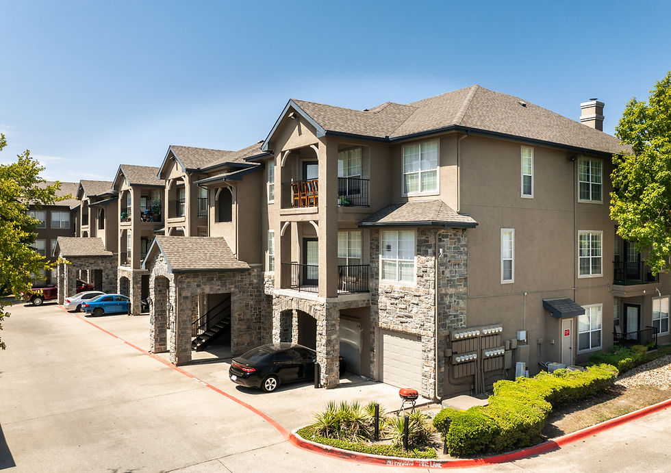
Sources:

• National Low Income Housing Coalition, The Gap: A Shortage of Affordable Homes, 2025 – highlighting a shortage of 7.1 million affordable rentals for extremely low-income Americans.

• Zillow Research, Press Release May 12, 2025: Showing renters need over $80k nationwide (and six-figure incomes in 8 major metros) to afford typical rents; Miami’s median rent equal to ~40% of local median income, while Austin’s is ~20%.

• RSM US, Workforce housing: The $1.8T opportunity for real estate investors (July 2025): Defining the affordability gap between subsidized and market-rate housing, and describing public-private strategies (like in Texas) to close it.

• City of Austin Housing and Planning Dept., FY2025 Income & Rent Limits: Detailing Austin’s HUD median income ($133,800) and affordable rent levels at various AMIs, illustrating how 60-80% AMI rents compare to market rents.

• Colorado Housing Finance Authority, Housing Affordability Gap White Paper (June 2025): Emphasizing the gap between development costs and income-supported financing, with examples of unit costs $250k–$300k and how land costs and construction type influence the gap

• CultureMap Austin, Rent affordability news (May 20, 2025): Reporting Zillow data that Austin renters need ~$68,840 to afford median rent, and are on average spending only ~20% of income on rent (versus ~30% nationally) – showing Austin’s relatively smaller gap at median.

• HUD User / Novogradac, FY 2025 Income Limits: Explaining the 2025 AMI update cap of 9.2% and that many areas hit this cap, with 71% of areas up over 5% – underscoring significant income changes that affect affordability calculations.

• Zillow Observed Rent Index Data (April/May 2025) – providing median rents and rent-to-income percentages for our focus cities (Austin, Miami, Phoenix, Raleigh, Denver, Atlanta), which we used to compute and compare Affordability Gap Indices across markets.